Molecular CISD
CISD Coefficients and amplitudes
Nomenclature:
Strings: the state decided by occupations, e.g., \(|001101\rangle\).
States: the state decided by applying excitation operators onto \(|\Phi_0\rangle = |HF\rangle\), e.g., \(a^\dagger_4 a_2 |\Phi_0\rangle\).
Coefficients: linear combination coefficient of strings.
Amplitudes: linear combination coefficients of states.
Note that \(a^\dagger_4 a_2 |\Phi_0\rangle = a^\dagger_4 a_2 a^\dagger_3 a^\dagger_2 a^\dagger_1 |-\rangle = - a^\dagger_4 a^\dagger_3 a^\dagger_1 |-\rangle = -|001101\rangle\). Therefore, one has to be careful with the sign changes going from states to strings or backward.
Representing a CISD wavefunction
In PySCF, there are three ways of representing a CISD wavefunction: (1) CISD coefficients, (2) FCI coefficients, and (3) CISD amplitudes.
CISD coefficients
The CISD coefficients \(\mathbf{v}\) are linear combination coefficients of the CISD strings,
where \(|s_i\rangle\) is a Slater determinant of a certain occupation pattern, e.g. \(|001011\rangle\).
The CISD coefficients \(\mathbf{v}\) are obtained by calling
cisd.kernel().:
myci = ci.UCISD(mf) # define myci object from mf
e_corr, cisdvec = myci.kernel() # perform CISD calculation
cisdvec is a 1D numpy array, corresponding to the coefficients
of strings, the order of elements in the civec is
where \(v_0\) is of length 1, \(v_{1\uparrow}\) and \(v_{1\downarrow}\) are of length \(N_\text{occ}N_\text{vir}\) (suppose the two spins have the same number of electrons), \(v_{2 \uparrow\downarrow}\) is of size \((N_\text{occ}N_\text{vir})^2\), \(v_{2\uparrow\uparrow}\) and \(v_{2\downarrow\downarrow}\) are of size \({N_\text{occ}\choose 2}{N_\text{vir}\choose 2}\). The orbital order of \(v_2\) is the asscending order of \(o_1o_2v_1v_2\), where \(o_2 > o_1\) and \(v_2 > v_1\).
FCI coefficients
One can turn the CISD coefficients into the FCI coefficients by calling:
fcivec = myci.to_fcivec(cisdvec)
which can be used as, e.g., an initial guess of the FCI calculation.
The reverse operation is:
cisdvec = myci.from_fcivec(fcivec)
CISD amplitudes
The amplitudes \(\mathbf{c}\) are coefficients of
where \(|\Phi_0\rangle\) is the Slater determinant for the ground state, and \(\hat{E}_i\) is an excitation operator of any order, e.g., \(\hat{E}_i = \hat{a}^\dagger_p \hat{a}_q \hat{a}^\dagger_r \hat{a}_s\). However, there is double counting in the sum of Eq. [eq:sum_amplitude], since \(\hat{a}^\dagger_p \hat{a}_q \hat{a}^\dagger_r \hat{a}_s\) and \(\hat{a}^\dagger_r \hat{a}_s\hat{a}^\dagger_p \hat{a}_q\) correspond to the same CI string.
In the following, we first give the PySCF syntax of deriving the amplitude, then evaluate the double counting in each type of excitation.
The CISD amplitudes can be derived by:
c0, c1, c2 = myci.cisdvec_to_amplitudes(cisdvec)
where c0 is the coefficient of
the HF GS; c1 is a list of arrays of spin-up and spin-down
amplitudes, respectively; c2 is a list of arrays of
\(\uparrow\uparrow\), \(\uparrow\downarrow\) and
\(\downarrow\downarrow\) excitations, respectively.
The reverse operation is:
cisdvec = myci.amplitudes_to_cisdvec(c0, c1, c2)
For the same spin double excitations, since
there is \(4\) fold degeneracy.
For cross-spin excitation, there is no double counting.
We first write the CISD vector in the FCI vector form (use
myci.to_fcivec(civec, norb, nelec) ), The order of FCI strings is:
string |
state |
|---|---|
0011 |
\(|HF\rangle\) |
1001 |
\(E_2^4\) |
0101 |
\(E_2^3\) |
1010 |
-\(E_1^4\) |
0110 |
-\(E_1^3\) |
1100 |
\(E_{12}^{34}\) |
In the following table, we present the coefficients for CI strings. We use the excitations to represent the strings for clarity, and keep in mind that the coefficients are with respect to strings not states. The corresponding FCI vector is
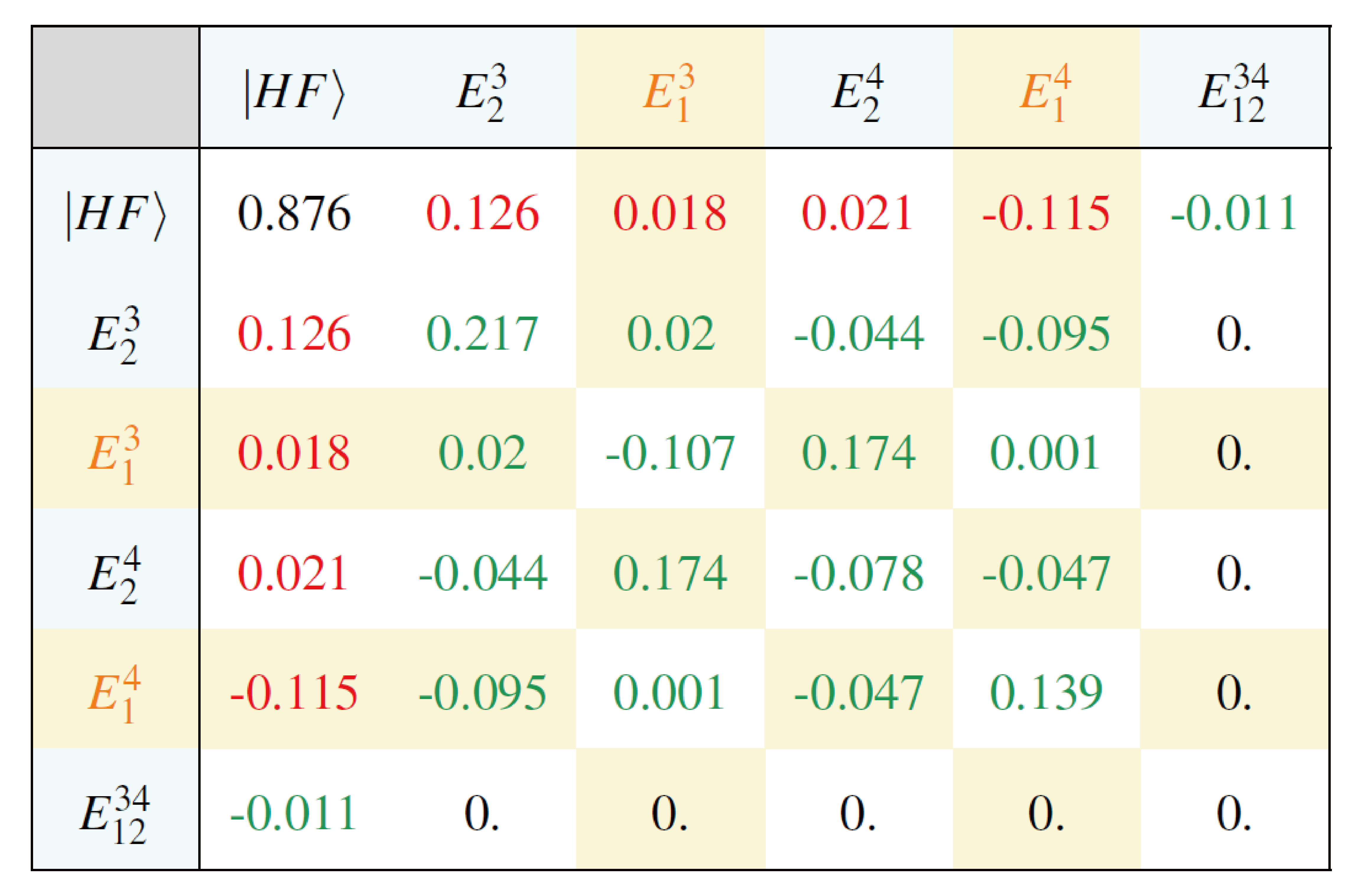
The rows are excitations for spin-up, and columns for spin-down. The red numbers corresponds to single excitations, and the green numbers are double excitations. Orange color corresponds to a minus sign.
The CISD amplitudes, i.e., the coefficient of the states, are derived by calling:
c0, c1, c2 = myci.cisdvec_to_amplitudes(civec)
Next, we examine the amplitudes c1 from single excitations. c1 is a 3D
array of size \((2, 2, 2)\), stands for (spin, occ, vir), and the
values are
Therefore, the amplitedes corresponding to \(C_1\) is
Next we examine double excitation amplitudes c2. The array
corresponding to c2 is of size (spin, nocc, nocc, nvir, nvir), where
the spin corresponds to
\(o^\alpha_1 o^\alpha_2 v^\alpha_1 v^\alpha_2\),
\(o^\alpha_1 o^\beta_2 v^\alpha_1 v^\beta_2\),
\(o^\beta_1 o^\beta_2 v^\beta_1 v^\beta_2\), where
\(\alpha = \uparrow\), \(\beta = \downarrow\), \(1\) and
\(2\) denotes two excitation pairs.
Therefore